flowchart LR
  H[CellBender .h5<br/>per sample] --> T[Threshold filter<br/>nFeature / nCount]
  T --> D[scDblFinder<br/>on filtered cells]
  D --> S[SCTransform<br/>per sample]
  S --> I[Integrate<br/>anchors]
  I --> P{{PCs}}
  P --> U{{UMAP<br/>settings}}
  U --> R{{Resolution}}
  R --> O[(Integrated object<br/>+ cluster QC)]
scRNA-seq QC and cluster calling (Seurat)
scRNA-seq
From CellBender-cleaned 10x counts to integrated, clustered Seurat objects: threshold filtering, doublet removal, SCTransform integration, and data-driven choices of PCs, UMAP settings and clustering resolution. Two R Markdown templates.
Overview
This picks up where the 10x → GeneExt → CellBender pipeline stops. It is two R Markdown files, run in order, interactively in RStudio (chunk by chunk, not knitted start to finish):
| Step | Template | Input → output |
|---|---|---|
| 1. QC | scrnaseq_1_QC.Rmd |
CellBender *_filtered.h5 per sample → QC_Files/SeuratObjectFiltered_<SPECIES>_<sample>.rds + QC summary table |
| 2. Cluster calling | scrnaseq_2_ClusterCalling.Rmd |
Filtered .rds files → <SPECIES>_integrated.rds with final clusters + diagnostics |
The hexagons are decision points. The template saves the diagnostics, then stops until you set the value yourself after looking at them. Nothing is picked automatically.
Inputs
- One CellBender
*_cellbender_output_filtered.h5per sample (empty droplets and ambient RNA already removed, so there is no separateemptyDrops()step). - A table of sample IDs plus one covariate per sample (genotype, treatment or batch). It is carried through so you can check that clusters aren’t driven by a single sample.
Software
R ≥ 4.3 with:
install.packages(c("tidyverse", "here", "Seurat", "scCustomize", "conflicted", "clustree",
                   "cluster", "clusterCrit", "FNN", "patchwork", "ggrastr"))
BiocManager::install(c("scDblFinder", "SingleCellExperiment", "glmGamPoi"))
Step 2 is the memory-hungry part (SCTransform + anchor integration). If it runs out of memory locally, run it on the cluster.
Run it
Download both templates into your project (an RStudio project, so
here()finds the root):Download
scrnaseq_1_QC.RmdDownloadscrnaseq_2_ClusterCalling.RmdFill in the Configuration chunk of step 1. Replace every
<fill in: ...>value; the next chunk stops if any are left:SPECIES <- "<fill in: species code, e.g. Gfas>" cellbender_dir <- here("<fill in: folder with CellBender .h5 files>") qc_out_dir <- here("<fill in: output folder, e.g. output/Gfas/QC>") sample_config <- tribble( ~sample_id, ~covariate, ~file, "<fill in: sample ID 1>", "<fill in: e.g. genotype 1>", "<fill in: sample1_..._filtered.h5>", ... )Also set
fix_feature_ids()(if your gene IDs need reformatting) andMITO_GENES(a pattern or list of mitochondrial gene IDs as they appear in the matrix; leaveNULLif your reference has none). The template prints the mito genes it found and stops if it found none.SYMBIONT_GENESworks the same way but only tracks the percentage (e.g. Symbiodiniaceae reads), it doesn’t filter.Run the pre-filter plots, then set thresholds. Look at
QC_Plots_<sample>.jpegbefore trusting the defaultqcMetricsThresholds; the defaults are the values used for G. fascicularis (and P. damicornis).Run the filter chunk and check
QC_Filtered_Summary_<SPECIES>.csv(see checks).Step 2: fill in its Configuration chunk (same
SPECIESand sample IDs), then run chunk by chunk, setting each decision value when you reach it.
What each step does
Step 1: QC
- Load each CellBender
.h5(scCustomize::Read_CellBender_h5_Mat), optionally reformat feature IDs, and addsample_id,covariateand the complexity scorelog10GenesPerUMI. - Pre-filter plots: violins of nFeature, nCount, log10GenesPerUMI (and percent_mito if available) with the thresholds drawn on.
- Threshold filter on nFeature and nCount (and percent_mito).
- Doublets:
scDblFinderon the cells that passed the filter (see known issues for why the order matters), then keep singlets. - Save one
.rdsper sample and a summary table.
Step 2: cluster calling
- SCTransform each sample (
glmGamPoi). percent_mito is not regressed out unless you setREGRESS_MITO <- TRUE; filtering high-mito cells in step 1 is the default. It also reports how many variable features the samples share. - Integrate with
SelectIntegrationFeatures→PrepSCTIntegration→FindIntegrationAnchors→IntegrateData(3,000 features; automatic retry at 2,000 if it runs out of memory). - PCs (decision 1): elbow plot, cumulative variance table, and PC gene-loading heatmaps in blocks of 9. Set
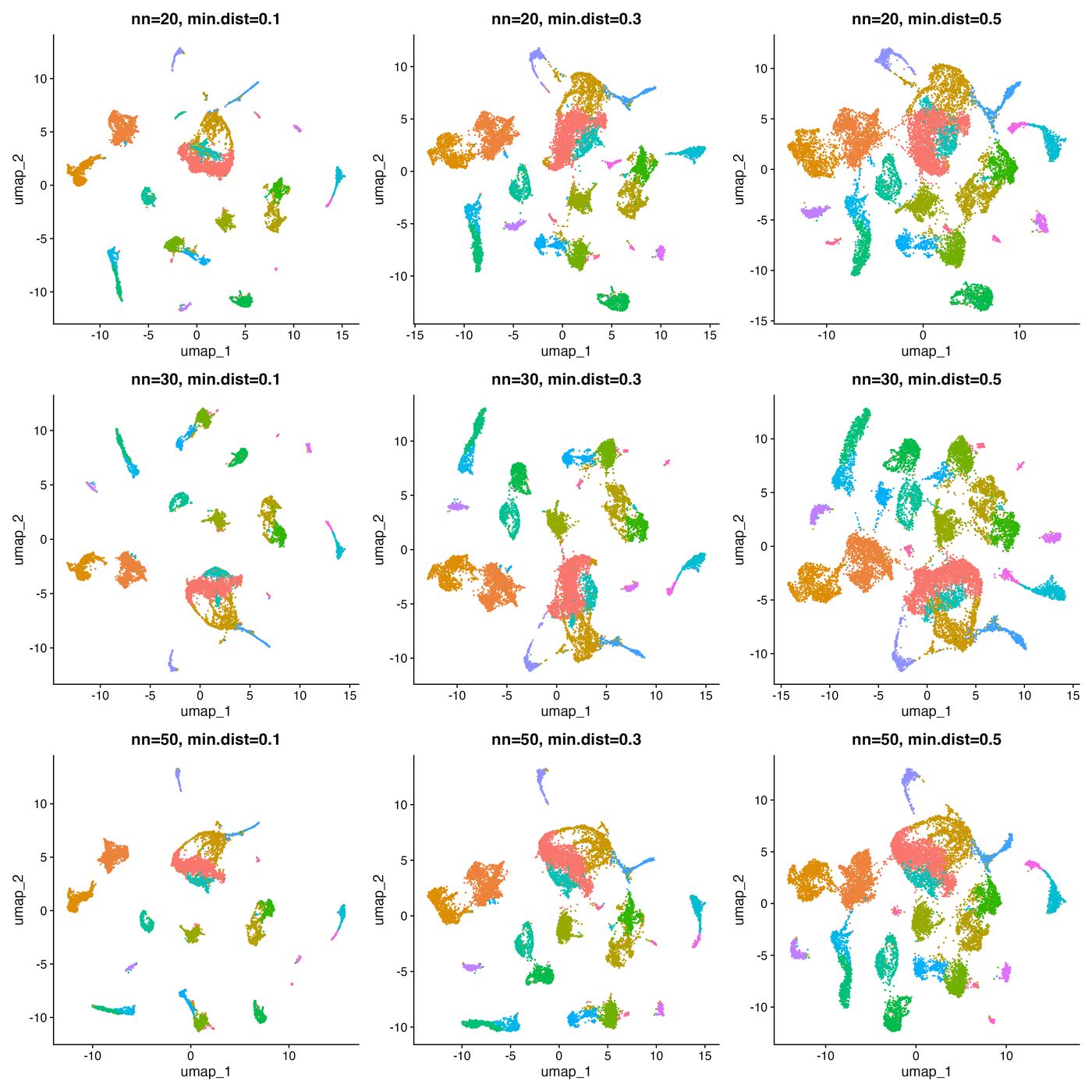
DIMS_FINAL. - UMAP settings (decision 2): a grid of
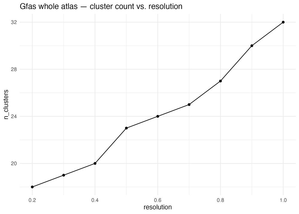
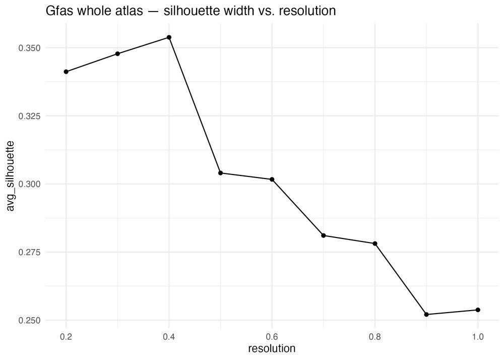
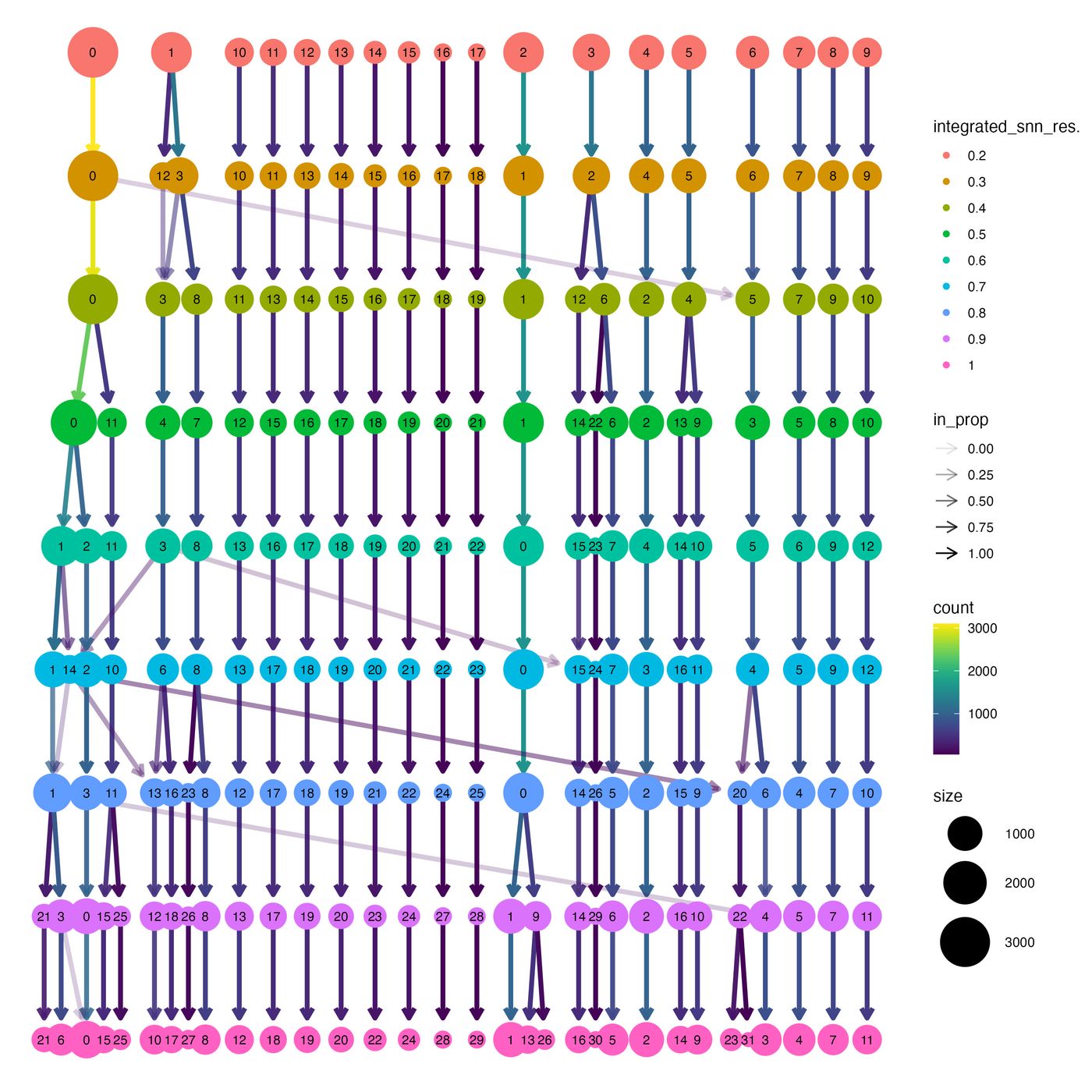
n.neighbors×min.distwith neighborhood preservation, Calinski–Harabasz, Davies–Bouldin, silhouette and covariate-mixing entropy. SetNN_FINALandMDIST_FINAL. - Resolution (decision 3): clusters at resolutions 0.2–1.0, with cluster count vs. resolution, clustree, silhouette vs. resolution, and one UMAP per resolution. Set
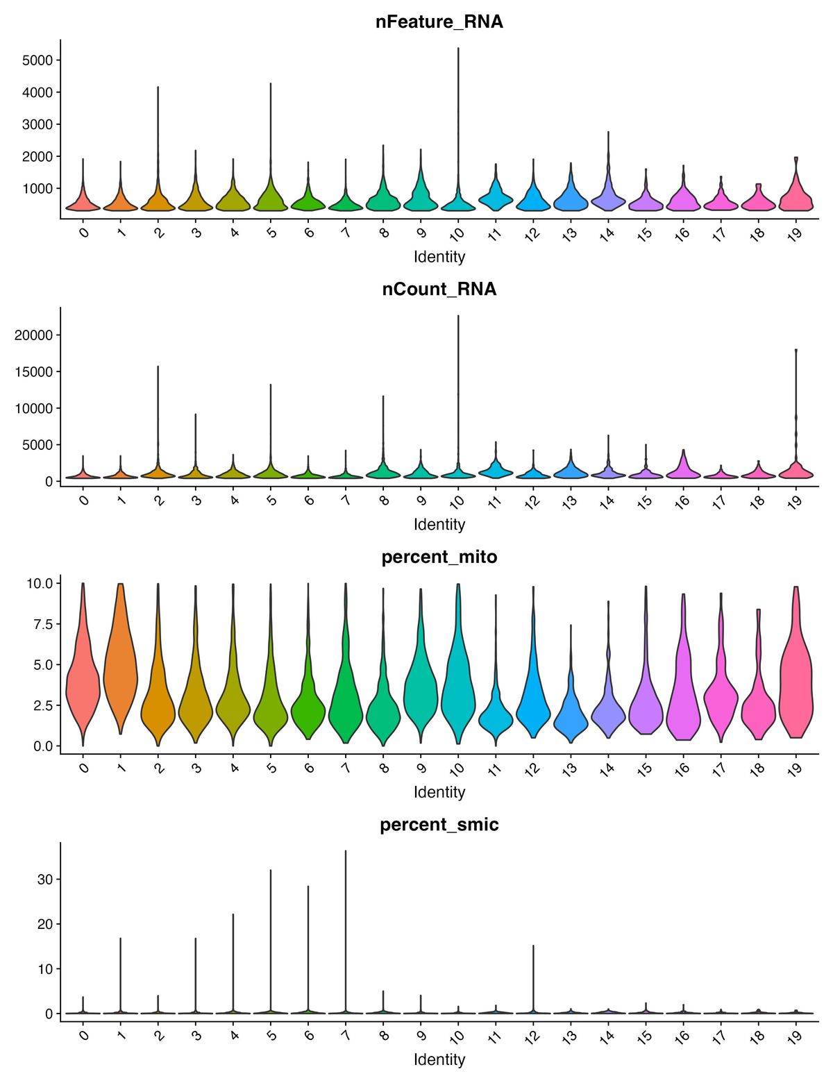
RES_FINAL. - Cluster QC: cells per cluster, % from the largest covariate level (flags < 50 cells or > 90% one level), QC violins per cluster, covariate stacked bar, and a UMAP split by covariate.
- Save
<SPECIES>_integrated.rdsand00_Finalised_Parameters.csv(the values you chose, for the record).
Checks before moving on
- Doublet rate roughly 0.5–10% for 10x data. Much higher usually means scDblFinder got unfiltered droplets, not that the data are bad.
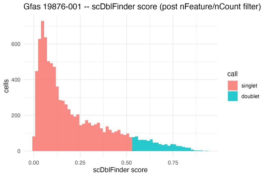
- Doublet score histogram: ideally the singlet/doublet cut sits in a trough. In low-UMI coral data there is often no clear second peak, and the cut falls in the right tail; that’s acceptable if the rate is reasonable, but don’t over-interpret individual calls.
- percent_mito actually varies (if you set
MITO_GENES). A column of zeros means the pattern matched nothing; see known issues. - Clusters flagged > 90% one sample: could be real biology (a genotype-specific state) or a batch effect. Look at their markers before naming them.
- Write down why you chose each decision value in your notebook entry.
00_Finalised_Parameters.csvonly records what was chosen.
Example: Galaxea fascicularis whole atlas
Three control colonies, each a different genotype and its own 10x lane (19876-001, 22901-001, 23362-001), August–September 2026. The CellBender reference combined the Galaxea nuclear genome, the published Galaxea mitogenome (Lu et al. 2024, GenBank ON341021) and Symbiodinium microadriaticum, so this dataset has real mitochondrial reads and symbiont reads to track.
QC
| Sample | Droplets in | After thresholds + mito | Doublets removed | Cells kept | Median genes | Median UMIs | Median % mito |
|---|---|---|---|---|---|---|---|
| 19876-001 | 27,481 | 9,202 | 915 (9.9%) | 8,287 | 509 | 741 | 3.4 |
| 22901-001 | 15,201 | 2,878 | 160 (5.6%) | 2,718 | 541 | 805 | 3.8 |
| 23362-001 | 14,701 | 3,914 | 256 (6.5%) | 3,658 | 503 | 752 | 2.0 |
| Total | 57,383 | 14,663 |
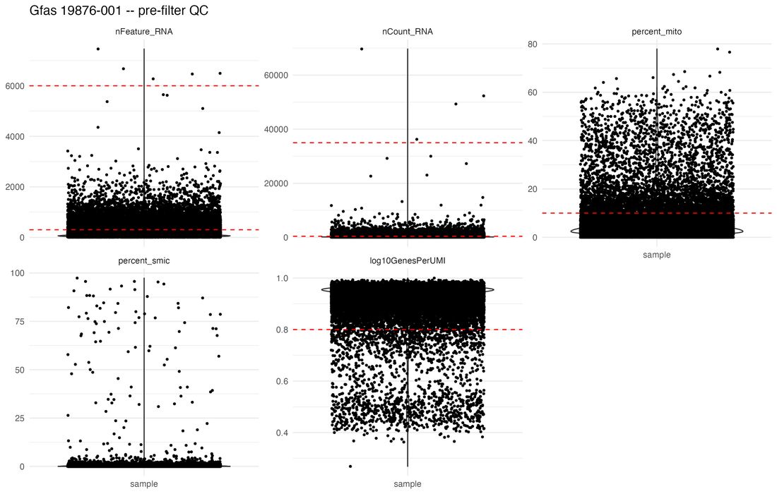
- Thresholds: 300–6,000 genes, 400–35,000 UMIs and ≤ 10% mito reads per cell. The gene and UMI bounds are the template defaults. The mito cap removed a further 0.3–7.5% of cells per sample on top of them.
- Mito genes: the mitogenome genes ended up with anonymous
gene_NIDs in the reference, so the 5 mito genes were identified from the data. They are highly expressed, detected in 33–89% of cells, tightly co-expressed with each other (r = 0.52–0.93) and consistent across samples. See Known issues. - Symbiont reads (
percent_smic) were tracked but not used to filter: 0.2–0.4% of library UMIs per sample. - Doublets: scDblFinder on the filtered cells, per sample, called 5.6–9.9%.
- Complexity: median log10GenesPerUMI 0.95 in all three samples.
Cluster calling
14,663 cells, integrated at 3,000 features. Shared variable features between sample pairs: Jaccard 0.43–0.50. The PC count was compared at 25 and 30, with the UMAP sweep run at both before one was chosen.
| Decision | Chosen | Why |
|---|---|---|
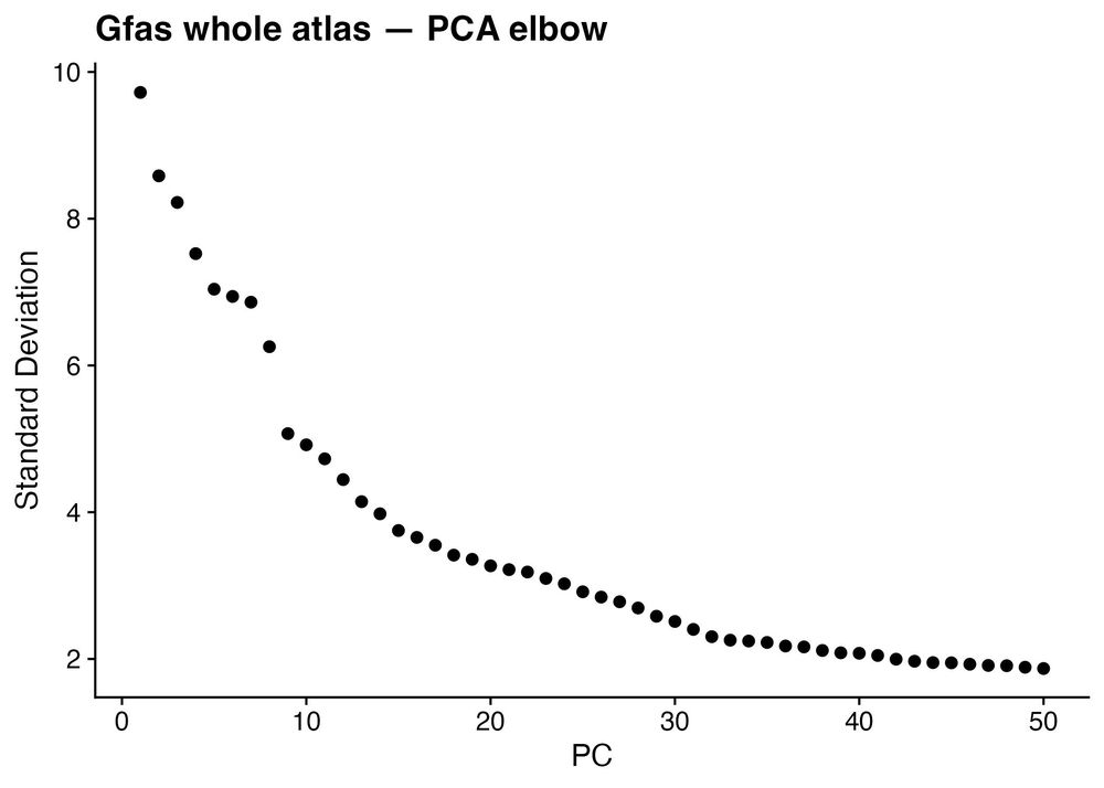
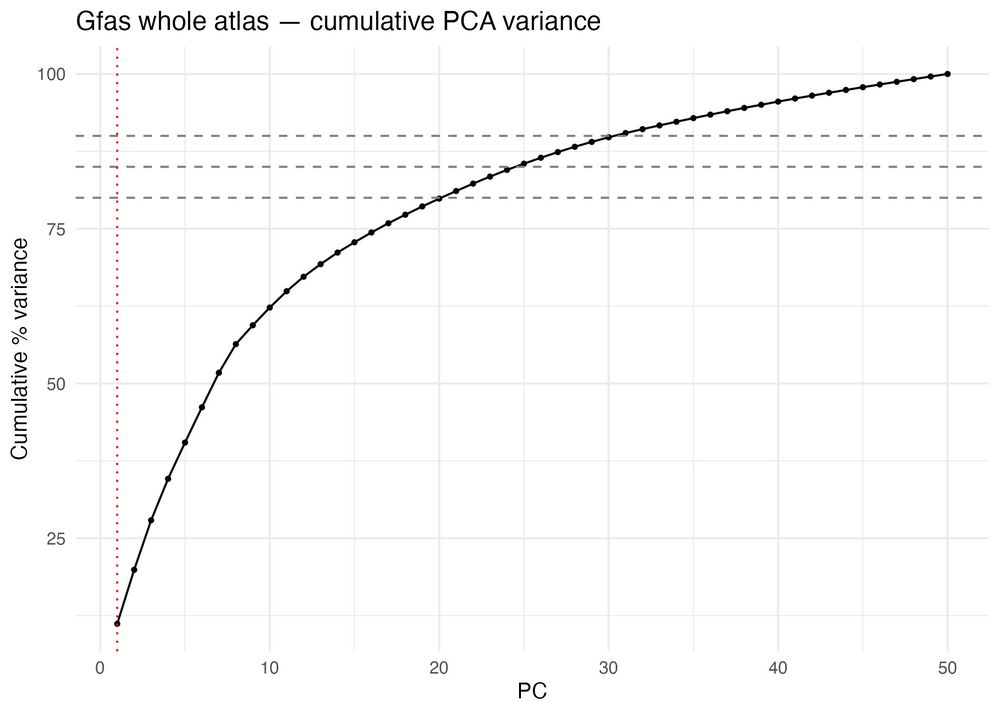
| PCs | 25 | No sharp elbow (steep drop through PC8, then a long taper). PC25 sits on the 85% cumulative-variance line (85.5%); PC30 (89.8%) was the first choice and was kept as a comparison. PC heatmaps showed nothing important lost by trimming to 25 |
| UMAP | n.neighbors 50, min.dist 0.3 | Neighborhood preservation was within 0.006 across the top settings (0.49–0.50). n.neighbors 50 gave the cleanest, best-separated layout in the 3 × 3 grid, while 20 looked fragmented |
| Resolution | 0.4 → 20 clusters | Silhouette peaks at 0.4 (0.354; 0.348 at 0.3, 0.304 at 0.5). Clustree shows 0.3 → 0.4 as mostly clean 1:1 refinements, while 0.4 → 0.5 brings several multi-way splits. The cluster count rises steadily (18 at 0.2 → 32 at 1.0) with no plateau |
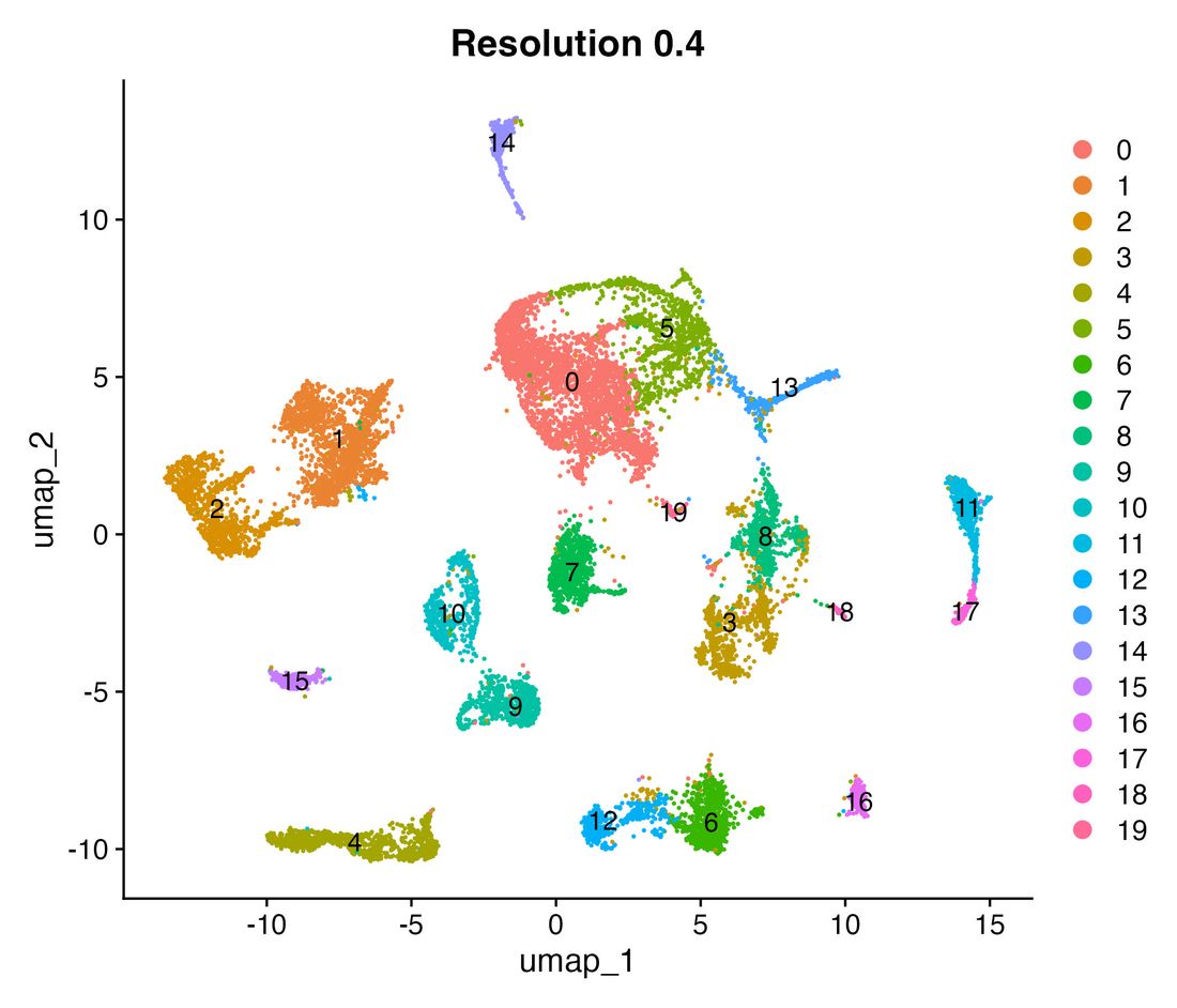
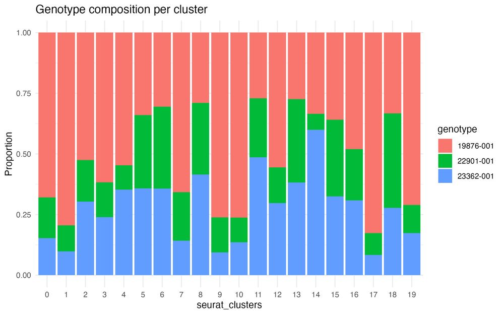
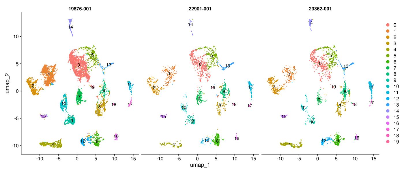
Cluster QC. No cluster was flagged: the smallest (cluster 19) has 69 cells, and the most genotype-skewed (cluster 17) is 82.7% one genotype. Clusters 0 and 1 carry higher mito (median ~4–5% vs ~2–3% elsewhere). Clusters 10 and 19 have long nCount tails (up to ~22,000 and ~18,000 UMIs), so they’re worth checking for doublets or stressed cells during annotation.
NoteOne library per genotype
Each genotype is a single 10x lane, so genotype and batch are confounded. A genotype-skewed cluster is a hypothesis to check against marker genes, not evidence of a genotype effect.
Known issues
WarningRun scDblFinder after filtering, not on the raw CellBender output
scDblFinder’s expected doublet rate grows with the number of cells it is given (~1% per 1,000 cells). On the unfiltered CellBender output (which still contains many marginal droplets) it called 20–39% of Pdam cells doublets. Run on the threshold-filtered cells it called a realistic 6.5–11%.
WarningCheck that your mitochondrial genes are actually counted
In the first Galaxea QC run, percent_mito was 0 in every cell, so the mito filter silently did nothing, and the symbiont counts were all zero too. The mito gene IDs had been written with underscores (gene_36687), but Seurat converts underscores to dashes on load (gene-36687), so the list matched no features. The same thing happened earlier with a pattern-based mito definition in an older Galaxea analysis.
Two fixes are now built into the step 1 template:
- write
MITO_GENESin the form the IDs take in the Seurat object (afterfix_feature_ids()and Seurat’s own_→-conversion); - the template prints the mito genes it found and stops if it found none.
A flat zero percent_mito violin is the giveaway.
If the mitogenome genes have uninformative IDs (Galaxea’s became gene_N when the references were combined), look for a small set of highly expressed, near-universally detected, tightly co-expressed features. Animal mitochondrial genes are transcribed together, so they correlate strongly. For Galaxea, 5 genes stood out, with a sharp drop in correlation after them (next best r = 0.27). 10x 3′ chemistry captures only some of the ~15 mitochondrial transcripts, so finding just a few is expected.
If your reference has no mito genes (e.g. P. damicornis), leave MITO_GENES <- NULL. log10GenesPerUMI is plotted as a mito-independent check for damaged or low-complexity droplets (reference line at 0.80, not used as a filter).
NoteGene IDs: underscores vs dashes
Seurat swaps _ for - in feature names and warns about it, so IDs like pdam_00025168 from GeneExt/CellBender become pdam-00025168. Pdam IDs are converted once at load time with fix_feature_ids() so the IDs match your functional annotation and ortholog tables.
Note
FindIntegrationAnchors runs out of memory
With Seurat v5 and 3,000 features this can fail with a memory error. The template retries at 2,000 features and records the number actually used in 00_Finalised_Parameters.csv.
NoteThe UMAP sweep doesn’t change the clusters
n.neighbors and min.dist only change the 2D picture; clusters come from the PCA neighbor graph. So in the Galaxea sweep, silhouette, Calinski–Harabasz, Davies–Bouldin and entropy were identical for every UMAP setting, and only neighborhood preservation varies. Treat this as a visualization choice.
NoteLow silhouette widths are normal here
Average silhouettes of 0.25–0.35 (Galaxea) look low but are typical for integrated scRNA-seq with many related cell states. Use it to compare resolutions (look for a peak or plateau), not as an absolute quality score.
How it connects
- Before: 10x Cell Ranger → GeneExt → CellBender produces the
.h5inputs. - After: clusters are annotated using functional annotation of each gene, and markers transferred from other species through OrthoFinder orthologs.
Full templates
scrnaseq_1_QC.Rmd
---
title: "scRNA-seq QC: CellBender counts -> QC-filtered Seurat objects"
subtitle: "Template from https://kevinhwong1.github.io/KevinHWong_Notebook/pipelines/scrnaseq-qc-clustering.html"
author: "<fill in: your name>"
date: "`r Sys.Date()`"
output:
  html_document:
    toc: true
    toc_float: true
    number_sections: true
---

<!--
STEP 1 OF 2 (QC). Next: scrnaseq_2_ClusterCalling.Rmd.

What this does, per sample:
  1. Load the CellBender-filtered .h5 (ambient RNA removed, empty droplets already dropped).
  2. Optionally fix feature IDs so they match your annotation tables.
  3. Plot nFeature / nCount / log10GenesPerUMI (and percent_mito if you have mitochondrial genes).
  4. Filter on nFeature / nCount (and percent_mito). Symbiont reads, if set, are tracked only.
  5. Detect doublets with scDblFinder ON THE FILTERED CELLS (see the note in that chunk), drop them.
  6. Save one filtered .rds per sample + a QC summary table.

Fill in every "<fill in: ...>" in the Configuration chunk. The first chunk after it stops if any
are left. Set thresholds AFTER looking at the pre-filter plots: the defaults are the values used
for Galaxea fascicularis and Pocillopora damicornis, not universal numbers.
-->

# Setup

```{r setup, include = FALSE}
knitr::opts_chunk$set(echo = TRUE, warning = TRUE, message = TRUE)
```

```{r libraries}
library(here)
library(tidyverse)
library(Seurat)
library(scCustomize)        # Read_CellBender_h5_Mat()
library(scDblFinder)        # BiocManager::install(c("scDblFinder", "SingleCellExperiment"))
library(SingleCellExperiment)
library(conflicted)

conflicts_prefer(
  dplyr::select, dplyr::filter, dplyr::count, dplyr::rename,
  base::intersect, base::union, base::setdiff,
  .quiet = TRUE
)
```

# Configuration

```{r config}
SPECIES <- "<fill in: species code, e.g. Gfas>"

# Folder with the CellBender *_filtered.h5 files, and where QC outputs should go
# (paths are relative to the project root found by here::here()).
cellbender_dir <- here("<fill in: folder with CellBender .h5 files, e.g. cellbender_output/Gfas>")
qc_out_dir     <- here("<fill in: output folder, e.g. output/Gfas/QC>")

# One row per sample. `covariate` is whatever distinguishes samples biologically or technically
# (genotype, treatment, batch...); it is carried into the clustering step to check mixing.
sample_config <- tribble(
  ~sample_id,                           ~covariate,                          ~file,
  "<fill in: sample ID 1>",             "<fill in: e.g. genotype 1>",        "<fill in: sample1_cellbender_output_filtered.h5>",
  "<fill in: sample ID 2>",             "<fill in: e.g. genotype 2>",        "<fill in: sample2_cellbender_output_filtered.h5>"
)
COVARIATE_NAME <- "genotype"   # what the covariate column means (used in plot labels)

# Optional: make feature IDs match your annotation tables. GeneExt/CellBender IDs for Pdam use
# underscores (pdam_00025168) while downstream tables use dashes (pdam-00025168).
# Use identity (function(x) x) to leave IDs unchanged.
fix_feature_ids <- function(x) gsub("_", "-", x)

# Optional mitochondrial filter. NULL = no mito genes in your reference (true for Pdam).
# Otherwise a regex matching mitochondrial gene IDs AS THEY APPEAR IN THE MATRIX (after fix_feature_ids),
# e.g. "^mt-", or a character vector of IDs. The load step stops if this matches no features --
# a pattern that silently matches nothing gives percent_mito = 0 for every cell.
# Galaxea example: c("gene-36687", "gene-24515", "gene-32266", "gene-5386", "gene-10331")
MITO_GENES <- NULL
max_percent_mito <- 10   # only used when MITO_GENES is set (10% for Galaxea)

# Optional symbiont (or other contaminant/organism) genes to TRACK, not filter: adds percent_symbiont
# per cell, a pre-filter plot panel and a column in the summary. Same format as MITO_GENES. NULL = skip.
SYMBIONT_GENES <- NULL

# QC thresholds -- check them against the pre-filter plots below before trusting them.
# Defaults = values used for G. fascicularis and P. damicornis (cross-checked against Cole et al.
# 2024 and Valadez-Ingersoll et al. 2025 for other cnidarians).
qcMetricsThresholds <- c(
  "min_nFeature_RNA" = 300,
  "max_nFeature_RNA" = 6000,
  "min_nCount_RNA"   = 400,
  "max_nCount_RNA"   = 35000
)
noveltyReferenceThreshold <- 0.80   # log10GenesPerUMI reference line: plotted, NOT used to filter

SEED <- 20260827
```

```{r check-config}
cfg_values <- c(SPECIES, cellbender_dir, qc_out_dir, unlist(sample_config))
stopifnot("Replace every '<fill in: ...>' value in the Configuration chunk first." =
            !any(grepl("<fill in", cfg_values, fixed = TRUE)))

sample_config <- sample_config %>% mutate(path = file.path(cellbender_dir, file))
stopifnot("One or more CellBender .h5 files not found -- check cellbender_dir and file names." =
            all(file.exists(sample_config$path)))
stopifnot("sample_id values must be unique." = !anyDuplicated(sample_config$sample_id))

qc_rds_dir <- file.path(qc_out_dir, "QC_Files")
dir.create(qc_rds_dir, recursive = TRUE, showWarnings = FALSE)

qcMetrics.tmp <- c("nFeature_RNA", "nCount_RNA", "log10GenesPerUMI",
                   if (!is.null(MITO_GENES)) "percent_mito",
                   if (!is.null(SYMBIONT_GENES)) "percent_symbiont")

# Resolve a pattern (length 1) or an ID list against the features actually in the object.
match_features <- function(genes, obj) {
  if (length(genes) == 1) grep(genes, rownames(obj), value = TRUE) else intersect(genes, rownames(obj))
}
sample_config
```

# Load CellBender-filtered counts

```{r load-objects}
# CellBender already removed empty droplets, so no separate emptyDrops() step.
sample.list <- pmap(sample_config, function(sample_id, covariate, file, path) {
  message("Loading ", sample_id, " ...")
  mat <- Read_CellBender_h5_Mat(path)
  rownames(mat) <- fix_feature_ids(rownames(mat))
  obj <- CreateSeuratObject(mat)

  obj$sample_id <- sample_id
  obj$covariate <- covariate

  # Complexity/novelty score: mito-independent sign of damaged / low-complexity droplets.
  obj$log10GenesPerUMI <- log10(obj$nFeature_RNA) / log10(obj$nCount_RNA)

  if (!is.null(MITO_GENES)) {
    mito_hits <- match_features(MITO_GENES, obj)
    if (length(mito_hits) == 0) {
      stop("MITO_GENES matches no features in ", sample_id, ". Check the pattern against ",
           "head(rownames(obj)), or set MITO_GENES <- NULL if your reference has no mito genes.")
    }
    message("  ", length(mito_hits), " mitochondrial features: ", paste(head(mito_hits, 5), collapse = ", "),
            if (length(mito_hits) > 5) ", ...")
    obj$percent_mito <- PercentageFeatureSet(obj, features = mito_hits)
  }

  if (!is.null(SYMBIONT_GENES)) {
    sym_hits <- match_features(SYMBIONT_GENES, obj)
    if (length(sym_hits) == 0) stop("SYMBIONT_GENES matches no features in ", sample_id, ".")
    obj$percent_symbiont <- PercentageFeatureSet(obj, features = sym_hits)
  }
  obj
})
names(sample.list) <- sample_config$sample_id

map_int(sample.list, ncol)
```

# QC diagnostic plots (pre-filter)

```{r qc-plots}
walk2(sample.list, names(sample.list), function(obj, sid) {
  plot_df <- obj@meta.data %>%
    select(all_of(qcMetrics.tmp)) %>%
    pivot_longer(everything(), names_to = "metric", values_to = "value") %>%
    mutate(metric = factor(metric, levels = qcMetrics.tmp))

  thresh_df <- tibble(
    metric    = str_replace(names(qcMetricsThresholds), "^(min|max)_", ""),
    threshold = unname(qcMetricsThresholds)
  ) %>%
    bind_rows(tibble(metric = "log10GenesPerUMI", threshold = noveltyReferenceThreshold)) %>%
    bind_rows(if (!is.null(MITO_GENES)) tibble(metric = "percent_mito", threshold = max_percent_mito)) %>%
    filter(metric %in% qcMetrics.tmp) %>%
    mutate(metric = factor(metric, levels = qcMetrics.tmp))

  p <- ggplot(plot_df, aes(x = "sample", y = value)) +
    geom_violin() +
    ggrastr::rasterise(geom_jitter(size = 0.5), dpi = 300) +
    facet_wrap(~metric, ncol = length(qcMetrics.tmp), scales = "free_y") +
    geom_hline(data = thresh_df, aes(yintercept = threshold), color = "red", linetype = "dashed") +
    labs(title = paste0(SPECIES, " ", sid, " -- pre-filter QC"), x = NULL, y = NULL) +
    theme_minimal(base_size = 11)

  ggsave(file.path(qc_out_dir, sprintf("QC_Plots_%s.jpeg", sid)),
         p, dpi = 300, width = 3.7 * length(qcMetrics.tmp), height = 4, units = "in")
})

cat("QC plots saved to:", qc_out_dir, "\n")
```

# Filter, remove doublets, save

```{r filter-and-save}
qc_summary <- pmap_dfr(sample_config, function(sample_id, covariate, file, path) {
  obj <- sample.list[[sample_id]]
  total_before <- ncol(obj)

  # Step 1: threshold filter.
  keep <- obj$nFeature_RNA >= qcMetricsThresholds["min_nFeature_RNA"] &
          obj$nFeature_RNA <= qcMetricsThresholds["max_nFeature_RNA"] &
          obj$nCount_RNA   >= qcMetricsThresholds["min_nCount_RNA"] &
          obj$nCount_RNA   <= qcMetricsThresholds["max_nCount_RNA"]
  if (!is.null(MITO_GENES)) keep <- keep & obj$percent_mito <= max_percent_mito
  obj_qc <- subset(obj, cells = colnames(obj)[keep])

  # Step 2: doublets. Run scDblFinder on the ALREADY-FILTERED cells. Its automatic expected doublet
  # rate scales with the number of cells it is given (~1% per 1,000 cells); running it on the raw
  # CellBender output (which still contains many marginal droplets) inflated the Pdam doublet rate
  # to 20-39%. On the filtered cells it was a realistic 6.5-11%.
  sce <- SingleCellExperiment(
    assays = list(counts = GetAssayData(obj_qc, assay = DefaultAssay(obj_qc), layer = "counts"))
  )
  set.seed(SEED)
  sce <- scDblFinder(sce)
  obj_qc$scDblFinder.class <- sce$scDblFinder.class
  obj_qc$scDblFinder.score <- sce$scDblFinder.score

  p_dbl <- ggplot(obj_qc@meta.data, aes(x = scDblFinder.score, fill = scDblFinder.class)) +
    geom_histogram(bins = 60, alpha = 0.85, position = "identity") +
    labs(title = paste0(SPECIES, " ", sample_id, " -- scDblFinder score (after threshold filter)"),
         x = "scDblFinder score", y = "cells", fill = "call") +
    theme_minimal(base_size = 11)
  ggsave(file.path(qc_out_dir, sprintf("Doublet_Score_%s.jpeg", sample_id)),
         p_dbl, dpi = 300, width = 6, height = 4, units = "in")

  # Step 3: keep singlets.
  cells_keep <- colnames(obj_qc)[obj_qc$scDblFinder.class == "singlet"]
  n_doublets <- ncol(obj_qc) - length(cells_keep)
  obj_filtered <- subset(obj_qc, cells = cells_keep)

  saveRDS(obj_filtered, file.path(qc_rds_dir, sprintf("SeuratObjectFiltered_%s_%s.rds", SPECIES, sample_id)))

  tibble(
    sample_id                   = sample_id,
    covariate                   = covariate,
    total_cells_before          = total_before,
    total_cells_after_qc_filter = ncol(obj_qc),
    n_doublets_removed          = n_doublets,
    pct_doublets                = round(100 * n_doublets / ncol(obj_qc), 2),
    total_cells_kept            = ncol(obj_filtered),
    pct_kept                    = round(100 * ncol(obj_filtered) / total_before, 1),
    median_nFeature             = median(obj_filtered$nFeature_RNA),
    median_nCount               = median(obj_filtered$nCount_RNA),
    median_log10GenesPerUMI     = round(median(obj_filtered$log10GenesPerUMI), 3),
    pct_below_novelty_reference = round(100 * mean(obj_filtered$log10GenesPerUMI < noveltyReferenceThreshold), 1),
    median_percent_mito         = if (!is.null(MITO_GENES)) round(median(obj_filtered$percent_mito), 2) else NA,
    median_percent_symbiont     = if (!is.null(SYMBIONT_GENES)) round(median(obj_filtered$percent_symbiont), 3) else NA
  )
})

write_csv(qc_summary, file.path(qc_out_dir, sprintf("QC_Filtered_Summary_%s.csv", SPECIES)))
qc_summary
```

<!--
CHECK BEFORE MOVING ON
- pct_doublets should be roughly 0.5-10% for 10x data. Much higher usually means scDblFinder was
  given too many (unfiltered) cells, not that the data are bad.
- In Doublet_Score_<sample>.jpeg the singlet/doublet boundary ideally sits in a trough. With low-UMI
  data there is often no second peak and the cut falls in the right tail; fine if the rate is sensible.
- Next: scrnaseq_2_ClusterCalling.Rmd reads QC_Files/SeuratObjectFiltered_<SPECIES>_<sample>.rds.
-->
scrnaseq_2_ClusterCalling.Rmd
---
title: "scRNA-seq cluster calling: integration, PCA, UMAP, clustering"
subtitle: "Template from https://kevinhwong1.github.io/KevinHWong_Notebook/pipelines/scrnaseq-qc-clustering.html"
author: "<fill in: your name>"
date: "`r Sys.Date()`"
output:
  html_document:
    toc: true
    toc_float: true
    number_sections: true
---

<!--
STEP 2 OF 2 (cluster calling). Input: QC_Files/SeuratObjectFiltered_<SPECIES>_<sample>.rds from
scrnaseq_1_QC.Rmd.

HOW TO USE THIS FILE
Run interactively, chunk by chunk -- do not knit start-to-finish. Several chunks are DECISION
POINTS: they save diagnostic plots/tables, then you set a parameter (DIMS_FINAL, NN_FINAL,
MDIST_FINAL, RES_FINAL) by reading those outputs. Later chunks stop with a clear message until the
parameter is set. Values used for the G. fascicularis atlas (3 samples, 14.7k cells) are given in comments as an
example, not a default.
-->

# Setup

```{r setup, include = FALSE}
knitr::opts_chunk$set(echo = TRUE, warning = TRUE, message = TRUE)
```

```{r libraries}
library(here)
library(tidyverse)
library(Seurat)
library(glmGamPoi)
library(conflicted)
library(clustree)
library(cluster)       # silhouette
library(clusterCrit)   # Calinski-Harabasz, Davies-Bouldin
library(FNN)            # neighborhood preservation (get.knn)
library(patchwork)

conflicts_prefer(
  dplyr::select, dplyr::filter, dplyr::count, dplyr::rename, dplyr::first,
  base::intersect, base::union, base::setdiff,
  purrr::map, purrr::discard,
  .quiet = TRUE
)

set.seed(1234)
```

# Configuration

```{r config}
SPECIES <- "<fill in: species code, same as in scrnaseq_1_QC.Rmd, e.g. Gfas>"

qc_rds_dir <- here("<fill in: QC output folder from step 1, e.g. output/Gfas/QC>", "QC_Files")
out_base   <- here("<fill in: output folder for clustering, e.g. output/Gfas/Seurat>")

# Sample IDs exactly as in step 1 (files are QC_Files/SeuratObjectFiltered_<SPECIES>_<sample_id>.rds)
sample_ids <- c("<fill in: sample ID 1>", "<fill in: sample ID 2>")
COVARIATE_NAME <- "genotype"   # what the covariate column from step 1 means (plot labels only)

N_VARIABLE_FEATURES <- 3000    # SCTransform / integration features (falls back to 2000 on memory errors)

# Regress percent_mito out in SCTransform? Default FALSE: filter high-mito cells in step 1 instead, so
# real biology correlated with mito content (e.g. metabolically active cell types) isn't removed.
# Consider TRUE if a cluster later looks mito-driven rather than biological.
REGRESS_MITO <- FALSE
```

```{r check-config}
stopifnot("Replace every '<fill in: ...>' value in the Configuration chunk first." =
            !any(grepl("<fill in", c(SPECIES, qc_rds_dir, out_base, sample_ids), fixed = TRUE)))

qc_out         <- file.path(out_base, "QC")
umap_sweep_dir <- file.path(qc_out, "UMAP_Sweep")
res_umap_dir   <- file.path(qc_out, "Resolution_UMAPs")
walk(c(out_base, qc_out, umap_sweep_dir, res_umap_dir), dir.create, recursive = TRUE, showWarnings = FALSE)

sample_config <- tibble(
  sample_id = sample_ids,
  path      = file.path(qc_rds_dir, sprintf("SeuratObjectFiltered_%s_%s.rds", SPECIES, sample_ids))
)
stopifnot("QC-filtered .rds files not found -- run scrnaseq_1_QC.Rmd first and check paths." =
          all(file.exists(sample_config$path)))
sample_config
```

# Load QC-filtered objects

```{r load-objects}
sample.list <- map(sample_config$path, readRDS)
names(sample.list) <- sample_config$sample_id

map_int(sample.list, ncol)
```

# Per-sample SCTransform

```{r sctransform}
# percent_mito is regressed only if REGRESS_MITO = TRUE and step 1 computed it.
sample.list <- map(sample.list, function(obj) {
  SCTransform(
    obj,
    method              = "glmGamPoi",
    variable.features.n = N_VARIABLE_FEATURES,
    vars.to.regress     = if (REGRESS_MITO && "percent_mito" %in% colnames(obj@meta.data)) "percent_mito" else NULL,
    verbose             = FALSE
  )
})
```

```{r variable-feature-overlap}
var_feats <- map(sample.list, VariableFeatures)

pairwise_overlap <- combn(names(var_feats), 2, function(pair) {
  a <- var_feats[[pair[1]]]; b <- var_feats[[pair[2]]]
  tibble(
    sample_a = pair[1], sample_b = pair[2],
    n_shared = length(intersect(a, b)),
    jaccard  = length(intersect(a, b)) / length(union(a, b))
  )
}, simplify = FALSE) %>% bind_rows()

all_shared <- Reduce(intersect, var_feats)
message("Variable features shared across all samples: ", length(all_shared))

write_csv(pairwise_overlap, file.path(qc_out, "00b_VariableFeature_Overlap.csv"))
pairwise_overlap
```

# Integration

```{r integration}
features <- SelectIntegrationFeatures(object.list = sample.list, nfeatures = N_VARIABLE_FEATURES)
nfeatures_used <- N_VARIABLE_FEATURES

sample.list.prepped <- PrepSCTIntegration(object.list = sample.list, anchor.features = features)

anchors <- tryCatch({
  FindIntegrationAnchors(
    object.list          = sample.list.prepped,
    normalization.method = "SCT",
    anchor.features      = features,
    dims                 = 1:30,
    k.anchor             = 5
  )
}, error = function(e) {
  # Known Seurat v5 memory issue (protocol Section 3.2 / 6): retry at nfeatures = 2000.
  message("FindIntegrationAnchors failed at nfeatures=", N_VARIABLE_FEATURES, " (", conditionMessage(e),
          "). Retrying at nfeatures=2000 -- known Seurat v5 memory issue.")
  nfeatures_used <<- 2000
  features2 <- SelectIntegrationFeatures(object.list = sample.list, nfeatures = 2000)
  sample.list.prepped2 <- PrepSCTIntegration(object.list = sample.list, anchor.features = features2)
  FindIntegrationAnchors(
    object.list          = sample.list.prepped2,
    normalization.method = "SCT",
    anchor.features      = features2,
    dims                 = 1:30,
    k.anchor             = 5
  )
})

combined <- IntegrateData(anchorset = anchors, normalization.method = "SCT")
DefaultAssay(combined) <- "integrated"

message("Integration complete. nfeatures used: ", nfeatures_used, " | cells: ", ncol(combined))
```

# PCA dimensionality — DECISION POINT

```{r pca}
combined <- RunPCA(combined, npcs = 50, verbose = FALSE)

p_elbow <- ElbowPlot(combined, ndims = 50) + ggtitle(paste(SPECIES, "— PCA elbow"))
ggsave(file.path(qc_out, "01_ElbowPlot.jpeg"), p_elbow, width = 7, height = 5)

stdev <- combined[["pca"]]@stdev
pct_var <- (stdev^2) / sum(stdev^2) * 100
cum_var <- cumsum(pct_var)

pc_variance_table <- tibble(
  PC = seq_along(pct_var),
  pct_var = pct_var,
  cum_var = cum_var
)
algorithmic_elbow <- which.min(diff(pct_var))
pc_at_80 <- min(which(cum_var >= 80))
pc_at_85 <- min(which(cum_var >= 85))
pc_at_90 <- min(which(cum_var >= 90))

message("Algorithmic elbow (max drop in per-PC variance): PC ", algorithmic_elbow)
message("Cumulative variance crossings — 80%: PC ", pc_at_80,
        " | 85%: PC ", pc_at_85, " | 90%: PC ", pc_at_90)

write_csv(pc_variance_table, file.path(qc_out, "02_CumulativeVariance.csv"))

p_cumvar <- ggplot(pc_variance_table, aes(PC, cum_var)) +
  geom_line() + geom_point(size = 0.8) +
  geom_hline(yintercept = c(80, 85, 90), linetype = "dashed", color = "grey50") +
  geom_vline(xintercept = algorithmic_elbow, linetype = "dotted", color = "red") +
  labs(y = "Cumulative % variance", title = paste(SPECIES, "— cumulative PCA variance")) +
  theme_minimal()
ggsave(file.path(qc_out, "02_CumulativeVariance.jpeg"), p_cumvar, width = 7, height = 5)

# PC gene-loading heatmaps in blocks of 9 -- confirm no early PC is dominated by a single gene
# family, and that PCs past your candidate cutoff aren't still biologically coherent.
pc_blocks <- split(1:50, ceiling(seq_along(1:50) / 9))
walk2(pc_blocks, seq_along(pc_blocks), function(dims_block, i) {
  jpeg(file.path(qc_out, sprintf("03_PCHeatmaps_block%02d.jpeg", i)),
       width = 1600, height = 1600, res = 150)
  DimHeatmap(combined, dims = dims_block, cells = 500, balanced = TRUE, fast = TRUE)
  dev.off()
})

pc_variance_table
```

```{r set-dims-final}
# ---- DECISION POINT ----
# Review 01_ElbowPlot.jpeg, 02_CumulativeVariance.jpeg/csv and the 03_PCHeatmaps_* blocks, then set
# DIMS_FINAL. Ignore the "algorithmic elbow" if it lands on PC1-2 (common with a steep PC1 drop).
# Galaxea example: DIMS_FINAL = 25 (85.5% cumulative variance; 30 was also tested).
DIMS_FINAL <- NA   # <-- SET ME

stopifnot("Set DIMS_FINAL above before continuing." = !is.na(DIMS_FINAL))
```

# UMAP parameter sweep — DECISION POINT

```{r umap-sweep, eval = !is.na(DIMS_FINAL)}
nn_grid   <- c(20, 30, 50)
mdist_grid <- c(0.1, 0.3, 0.5)
grid <- expand_grid(nn = nn_grid, mdist = mdist_grid)

DefaultAssay(combined) <- "integrated"

max_cells_metrics <- min(3000, ncol(combined))
metric_cells <- sample(colnames(combined), max_cells_metrics)

pca_emb <- Embeddings(combined, "pca")[metric_cells, 1:DIMS_FINAL]

sweep_results <- pmap(grid, function(nn, mdist) {
  combined <- RunUMAP(combined, dims = 1:DIMS_FINAL, n.neighbors = nn, min.dist = mdist,
                       verbose = FALSE)
  umap_emb <- Embeddings(combined, "umap")[metric_cells, ]

  # Neighborhood preservation: fraction of true k-NN (PCA space) recovered in UMAP space.
  k <- 30
  knn_pca  <- get.knn(pca_emb,  k = k)$nn.index
  knn_umap <- get.knn(umap_emb, k = k)$nn.index
  preservation <- mean(map_dbl(seq_len(nrow(knn_pca)), function(i) {
    length(intersect(knn_pca[i, ], knn_umap[i, ])) / k
  }))

  # Cluster quality at a fixed placeholder resolution (0.5) -- cross-grid comparison only, NOT the
  # final resolution decision (that's Section 3.5 below).
  combined <- FindNeighbors(combined, dims = 1:DIMS_FINAL, verbose = FALSE)
  combined <- FindClusters(combined, resolution = 0.5, verbose = FALSE)
  clust_sub <- combined$seurat_clusters[metric_cells]

  crit <- intCriteria(pca_emb, as.integer(clust_sub), c("Calinski_Harabasz", "Davies_Bouldin"))
  sil <- silhouette(as.integer(clust_sub), dist(pca_emb))
  avg_sil <- mean(sil[, "sil_width"])

  # Covariate mixing entropy per cluster, normalized to [0,1] (1 = perfectly mixed).
  covar_sub <- combined$covariate[metric_cells]
  n_cat <- length(unique(covar_sub))
  entropy_by_cluster <- tapply(covar_sub, clust_sub, function(x) {
    p <- table(x) / length(x)
    -sum(p * log(p)) / log(n_cat)
  })
  mean_entropy <- mean(entropy_by_cluster, na.rm = TRUE)

  p_umap <- DimPlot(combined, reduction = "umap", group.by = "seurat_clusters") +
    ggtitle(sprintf("nn=%d, min.dist=%.1f", nn, mdist)) +
    theme(legend.position = "none")

  list(
    metrics = tibble(
      n_neighbors = nn, min_dist = mdist,
      neighborhood_preservation = preservation,
      calinski_harabasz = crit$calinski_harabasz,
      davies_bouldin = crit$davies_bouldin,
      avg_silhouette = avg_sil,
      mean_covariate_entropy = mean_entropy
    ),
    plot = p_umap
  )
})

umap_sweep_metrics <- bind_rows(map(sweep_results, "metrics"))
write_csv(umap_sweep_metrics, file.path(umap_sweep_dir, "umap_sweep_metrics.csv"))

p_grid <- wrap_plots(map(sweep_results, "plot"), ncol = 3)
ggsave(file.path(umap_sweep_dir, "umap_sweep_grid.jpeg"), p_grid, width = 15, height = 15)

umap_sweep_metrics
```

```{r set-umap-final}
# ---- DECISION POINT ----
# Review umap_sweep_metrics.csv and umap_sweep_grid.jpeg. Prioritize neighborhood_preservation when
# metrics disagree, then prefer clean, round (not smeared) clusters. n.neighbors / min.dist only change
# the 2D layout -- clusters come from the PCA graph -- so this is a visualization choice. With few
# samples, don't over-weight mean covariate entropy.
# Galaxea example: NN_FINAL = 50, MDIST_FINAL = 0.3 (cleanest layout; preservation within 0.006 of the top).
NN_FINAL    <- NA   # <-- SET ME
MDIST_FINAL <- NA   # <-- SET ME

stopifnot("Set NN_FINAL and MDIST_FINAL above before continuing." =
            !is.na(NN_FINAL) && !is.na(MDIST_FINAL))

combined <- RunUMAP(combined, dims = 1:DIMS_FINAL, n.neighbors = NN_FINAL, min.dist = MDIST_FINAL,
                     verbose = FALSE)
```

# Clustering resolution sweep — DECISION POINT

```{r resolution-sweep, eval = !is.na(NN_FINAL)}
combined <- FindNeighbors(combined, dims = 1:DIMS_FINAL, verbose = FALSE)

res_seq <- seq(0.2, 1.0, by = 0.1)
combined <- FindClusters(combined, resolution = res_seq, verbose = FALSE)

res_cols <- grep("^integrated_snn_res\\.", colnames(combined@meta.data), value = TRUE)

# 1. Cluster count vs. resolution
cluster_counts <- tibble(
  resolution = res_seq,
  n_clusters = map_dbl(res_cols, ~ length(unique(combined@meta.data[[.x]])))
)
write_csv(cluster_counts, file.path(qc_out, "cluster_count_vs_resolution.csv"))

p_counts <- ggplot(cluster_counts, aes(resolution, n_clusters)) +
  geom_line() + geom_point() +
  labs(title = paste(SPECIES, "— cluster count vs. resolution")) +
  theme_minimal()
ggsave(file.path(qc_out, "05_ClusterCount_vs_Resolution.jpeg"), p_counts, width = 7, height = 5)

# 2. Clustree
p_clustree <- clustree(combined, prefix = "integrated_snn_res.")
ggsave(file.path(qc_out, "06_Clustree.jpeg"), p_clustree, width = 10, height = 10)

# 3. Silhouette width vs. resolution (subsampled, PCA-space distances)
pca_emb_full <- Embeddings(combined, "pca")[metric_cells, 1:DIMS_FINAL]
dist_full <- dist(pca_emb_full)

silhouette_by_res <- map_dbl(res_cols, function(col) {
  clust_sub <- combined@meta.data[metric_cells, col]
  if (length(unique(clust_sub)) < 2) return(NA_real_)
  mean(silhouette(as.integer(as.character(clust_sub)) + 1L, dist_full)[, "sil_width"])
})
silhouette_table <- tibble(resolution = res_seq, avg_silhouette = silhouette_by_res)
write_csv(silhouette_table, file.path(qc_out, "silhouette_vs_resolution.csv"))

p_sil <- ggplot(silhouette_table, aes(resolution, avg_silhouette)) +
  geom_line() + geom_point() +
  labs(title = paste(SPECIES, "— silhouette width vs. resolution")) +
  theme_minimal()
ggsave(file.path(qc_out, "07_Silhouette_vs_Resolution.jpeg"), p_sil, width = 7, height = 5)

# Per-resolution UMAP panels for visual/biological-interpretability review
walk(res_cols, function(col) {
  res_label <- sub("integrated_snn_res\\.", "", col)
  p <- DimPlot(combined, reduction = "umap", group.by = col, label = TRUE) +
    ggtitle(paste0("Resolution ", res_label))
  ggsave(file.path(res_umap_dir, sprintf("resolution_%s.jpeg", res_label)),
         p, width = 7, height = 6)
})

cluster_counts
```

```{r set-res-final}
# ---- DECISION POINT ----
# Review the plateau in 05_ClusterCount_vs_Resolution.jpeg, stable ("quiet") levels in 06_Clustree.jpeg,
# the peak/plateau in 07_Silhouette_vs_Resolution.jpeg, and whether clusters in Resolution_UMAPs/ look
# biologically sensible. Resolutions tested: 0.2-1.0 in steps of 0.1.
# Galaxea example: RES_FINAL = 0.4 (20 clusters; silhouette peak, clean 1:1 splits from 0.3).
RES_FINAL <- NA   # <-- SET ME

stopifnot("Set RES_FINAL above before continuing." = !is.na(RES_FINAL))

res_col_values <- as.numeric(sub("integrated_snn_res\\.", "", res_cols))
match_idx <- which(abs(res_col_values - RES_FINAL) < 1e-6)
stopifnot("RES_FINAL does not match any resolution column that was actually computed above." =
            length(match_idx) == 1)
final_res_col <- res_cols[match_idx]

combined$seurat_clusters <- combined@meta.data[[final_res_col]]
Idents(combined) <- "seurat_clusters"

message("Final clustering: ", length(unique(combined$seurat_clusters)), " clusters at resolution ",
        RES_FINAL)
```

# Cluster QC diagnostics

```{r cluster-qc, eval = !is.na(RES_FINAL)}
# Cell counts per cluster per covariate level -- flag <50 cells or >90% from one level.
cluster_covariate_counts <- combined@meta.data %>%
  count(seurat_clusters, covariate) %>%
  group_by(seurat_clusters) %>%
  mutate(total = sum(n), pct = n / total) %>%
  ungroup()

cluster_flags <- cluster_covariate_counts %>%
  group_by(seurat_clusters) %>%
  summarise(
    total_cells = first(total),
    max_covariate_pct = max(pct),
    flag_low_n = total_cells < 50,
    flag_covariate_skew = max_covariate_pct > 0.90,
    .groups = "drop"
  )
write_csv(cluster_flags, file.path(qc_out, "cluster_qc_flags.csv"))
write_csv(cluster_covariate_counts, file.path(qc_out, "cluster_covariate_counts.csv"))

if (any(cluster_flags$flag_low_n | cluster_flags$flag_covariate_skew)) {
  message("Clusters flagged for review before Stage B annotation:")
  print(filter(cluster_flags, flag_low_n | flag_covariate_skew))
}

qc_feats <- intersect(c("nFeature_RNA", "nCount_RNA", "log10GenesPerUMI", "percent_mito", "percent_symbiont"), colnames(combined@meta.data))
p_qc_violin <- VlnPlot(combined, features = qc_feats, group.by = "seurat_clusters", pt.size = 0, ncol = 1)
ggsave(file.path(qc_out, "cluster_qc_violins.jpeg"), p_qc_violin, width = 10, height = 8)

# Covariate mixing -- stacked bar + split UMAP
p_stack <- ggplot(cluster_covariate_counts, aes(seurat_clusters, pct, fill = covariate)) +
  geom_col() +
  labs(title = paste(COVARIATE_NAME, "composition per cluster"), y = "Proportion", fill = COVARIATE_NAME) +
  theme_minimal()
ggsave(file.path(qc_out, "cluster_covariate_stackedbar.jpeg"), p_stack, width = 8, height = 5)

p_split <- DimPlot(combined, reduction = "umap", split.by = "covariate", label = TRUE)
ggsave(file.path(qc_out, "umap_split_by_covariate.jpeg"), p_split, width = 6 * length(unique(combined$covariate)), height = 6)

cluster_flags
```

# Save finalized parameters and pre-annotation object

```{r save-outputs, eval = !is.na(RES_FINAL)}
finalised_params <- tibble(
  n_samples = nrow(sample_config),
  species = SPECIES,
  n_cells = ncol(combined),
  nfeatures_used = nfeatures_used,
  dims_final = DIMS_FINAL,
  nn_final = NN_FINAL,
  mdist_final = MDIST_FINAL,
  res_final = RES_FINAL,
  n_clusters_final = length(unique(combined$seurat_clusters)),
  date = as.character(Sys.Date())
)
write_csv(finalised_params, file.path(qc_out, "00_Finalised_Parameters.csv"))

saveRDS(combined, file.path(out_base, sprintf("%s_integrated.rds", SPECIES)))

finalised_params
```

<!--
NEXT STEPS
1. Check that each DECISION POINT value is justified by the diagnostics (and note why in your notebook).
2. Clusters flagged in cluster_qc_flags.csv (<50 cells, or >90% from one covariate level) need a look
   before annotation.
3. <SPECIES>_integrated.rds is the input to cluster annotation.
-->
References
- Hao Y et al. 2024. Dictionary learning for integrative, multimodal and scalable single-cell analysis (Seurat v5). Nature Biotechnology 42:293–304.
- Germain P-L et al. 2021. Doublet identification in single-cell sequencing data using scDblFinder. F1000Research 10:979.
- Hafemeister C & Satija R 2019. Normalization and variance stabilization of single-cell RNA-seq data using regularized negative binomial regression. Genome Biology 20:296.
- Zappia L & Oshlack A 2018. Clustering trees: a visualization for evaluating clusterings at multiple resolutions. GigaScience 7:giy083.
- Fleming SJ et al. 2023. Unsupervised removal of systematic background noise from droplet-based single-cell experiments using CellBender. Nature Methods 20:1323–1335.
Changelog
| Date | Change |
|---|---|
| 2026-10-06 | Galaxea whole atlas (3 genotypes) used as the worked example for QC and cluster calling; mito-gene check; optional mito regression and symbiont tracking |
| 2026-10-05 | Generic templates (config chunk, covariate column, optional mito) and this page |
| 2026-08-27 | P. damicornis whole atlas: decision-point workflow, cluster QC flags |
| 2026-06 | G. fascicularis 6-sample integrated atlas (genotype × treatment), checked against the control-only atlas |
| 2026-08 | scDblFinder moved after threshold filtering |