SATURN: ESM-1b vs three ESMC-600M embedding sets (raw, rescaled, post-norm) in four species
- Four gene-embedding sets are now compared:
- ESM-1b;
- ESMC-600M exactly as first delivered (“raw”);
- the same ESMC vectors set to equal length (“rescaled”);
- a second ESMC export from Ingrid Miranda Perez (“post-norm”, Oct 16–19), taken after the model’s final normalization layer instead of before it.
- How they are compared:
- on the embeddings alone, before SATURN: vector length, geometry, and whether each gene’s most similar gene in another species is a true ortholog;
- at the macrogene level: SATURN’s gene groups scored against eggNOG orthologous groups.
- The new post-norm export is the weakest of the four on the most-similar-gene test:
- The post-norm vectors are more collapsed and more species-specific: about 3 effective dimensions vs 10 for ESM-1b, and more variance explained by species (Table 6).
- Rescaling the first export changed vector lengths but not directions, and helped little: 34% → 36% here; macrogene recall 0.15 → 0.16 on Oct 8.
- So both ways of reading ESMC’s last layer, before and after its final normalization, fall below ESM-1b. Intermediate layers have not been tested. The ESMC paper (Candido et al. 2026) finds functional information peaks in intermediate layers, not the last one, so this is the obvious next test.
This entry pulls together the ESM-1b vs ESMC comparisons of Oct 6, Oct 8 and Oct 9, and adds the second ESMC export. Everything here uses the four original species (Mnemiopsis, oyster, Ciona, zebrafish).
Key terms
| Term | Meaning here |
|---|---|
| Protein language model (pLM) | A neural network trained to predict masked amino acids. On the way it learns a numerical description of each residue. |
| Embedding | One vector per protein, the average of the per-residue vectors from one layer of the pLM (mean pooling). SATURN uses one per gene, averaging the gene’s isoforms. |
| Extraction | The choices made when pulling an embedding out of a model: which layer, whether before or after the final normalization step, how residues are averaged, how long proteins are cut. Same model + different extraction = different embeddings. |
| LayerNorm | A normalization step inside transformer models. For each residue separately, it shifts and scales that residue’s vector to mean 0 and standard deviation 1 across its 1,152 numbers, then multiplies each dimension by a learned weight and adds a learned offset. ESMC ends with one, just before its output (section 1.1; Candido et al. 2026, Appendix A.1.1). |
| Hidden states / residual stream | The per-residue vectors passed from one transformer block to the next. The last block’s output, before the final LayerNorm, is what the first ESMC export used. |
| Vector length (L2 norm) | √(sum of squared values). For similarity, the direction of a vector carries the protein information; length mostly reflects the extraction. |
| Most-similar-gene test (hit@1) | For each gene in species A, take the most similar gene in species B and check whether both are in the same orthologous group. hit@10 = a true ortholog among the 10 most similar. Averaged over all 12 directed species pairs. No SATURN involved. |
| Euclidean / cosine | Two ways to measure similarity. Euclidean uses length and direction (what SATURN’s clustering sees); cosine uses direction only. |
| Effective dimensions (participation ratio) | Roughly how many independent directions the embeddings actually use. Low = most genes differ along only a few axes. |
| Species R² | Share of embedding variance explained by species identity alone. High = genes cluster by species before function. |
| Orthologous group (OG) | Genes descended from one ancestral gene. Two independent references: eggNOG Metazoa OGs, and OrthoFinder orthogroups computed from our four proteomes (Oct 15). |
| z-score / top-PC removal (abtt) | Standard fixes: z-score rescales every dimension to equal spread; all-but-the-top removes the 1–3 strongest directions shared by all proteins. |
1. The four embedding sets
ESM-1b vs ESMC: different models.
- ESM-1b (Rives et al. 2021) is SATURN’s default.
- 650 million parameters, 33 layers, 1,280 numbers per protein.
- Trained on UniRef50.
- Reads up to 1,022 residues.
- ESM C 600M (EvolutionaryScale 2024; described in full in Candido et al. 2026) is a newer model of similar size.
- 36 layers, 1,152 numbers per protein (Candido et al. 2026, Table S1).
- Trained on ~2.8 billion sequences vs ~50 million for ESM2, mostly metagenomic (JGI, MGnify) plus UniRef. Training ran in two stages: first 512-token context weighted to metagenomes, then 2,048-token context weighted to UniRef (Table S2–S3).
- Updated architecture: pre-norm transformer blocks, rotary position embeddings, and a final LayerNorm after the last block (Appendix A.1.1).
- Collaborators proposed it as the stronger model. On contact prediction, ESMC 600M matches ESM2-3B (Candido et al. 2026, Fig. 1C). The paper does not compare it with ESM-1b, nor test cross-species ortholog retrieval from mean-pooled final-layer vectors, which is what SATURN uses.
The three ESMC sets: one model, three extractions.
| ESM-1b | ESMC raw | ESMC rescaled | ESMC post-norm | |
|---|---|---|---|---|
| Model | ESM-1b 650M | ESM C 600M | ESM C 600M | ESM C 600M |
| Who extracted | us, fair-esm |
Ingrid, FANTASIA v4.1.1, checkpoint esmc_600m, fp32 (Sep 23–24) |
derived from raw (05e) |
Ingrid, standalone script, esmc_600m, fp32 (Oct 16–19) |
| Layer / normalization | final layer (33), after ESM-1b’s final LayerNorm | output of the final transformer block (hidden_states[-1], stored as layer_0), before ESMC’s final LayerNorm |
same as raw | output of the final transformer block after ESMC’s final LayerNorm |
| Averaging over residues | mean, start/end tokens excluded | mean, start/end tokens excluded | same as raw | mean, start/end tokens excluded |
| Post-processing | none | none | each vector divided by its length, × 17.665 (mean ESM-1b length) | none |
| Longest protein used | first 1,022 residues | first 2,000 residues (no windowing) | same as raw | first 2,000 residues (no windowing) |
| Vector length, HV genes | 16.3–19.6 | 1,718–8,902 | 17.7 (all equal) | 0.70–1.95 |
| Per gene | isoforms averaged (Mnemiopsis: longest isoform) | same | same | same |
- Rescaled is raw with the length removed. Its directions are identical to raw, so every cosine (direction-only) result is the same for the two.
- Post-norm is not just raw rescaled. Its directions differ: cosine results drop from 36% to 29% (Table 7). Section 1.1 explains why.
- Truncation is the same for all three ESMC sets (2,000 residues, inside ESMC’s 2,048-token training context; Candido et al. 2026, Table S3; 1–4% of proteins are longer). It differs from ESM-1b (1,022), but can’t explain differences between the ESMC sets.
1.1 What “post-norm” means
ESMC, like ESM-1b, processes a protein as a stack of transformer blocks. Each block updates one 1,152-number vector per residue. After the last block comes one more step, a final LayerNorm, and its output is what the model’s own prediction head uses (Candido et al. 2026, Appendix A.1.1: each block normalizes its input and adds its output back to the residual stream, so the stream itself is never normalized until this final step). A protein embedding is made by averaging the per-residue vectors over the protein. The question is which per-residue vectors are averaged.
| Per-residue vectors averaged | In words | |
|---|---|---|
| ESMC raw (FANTASIA) | output of the last block, before the final LayerNorm | the “residual stream” as it leaves the last block |
| ESMC post-norm | the same vectors after the final LayerNorm | what the model hands to its output head |
| ESM-1b (ours) | after ESM-1b’s final LayerNorm | the standard fair-esm extraction |
What the final LayerNorm does. It works on each residue’s vector separately:
- subtract that vector’s own mean and divide by its own standard deviation, so its 1,152 numbers have mean 0 and SD 1;
- multiply each of the 1,152 dimensions by a learned weight, and add a learned offset.
Why post-norm is not the same as rescaling raw:
- Order of operations. The normalization happens per residue, before averaging. Rescaling divides the averaged vector by its length afterwards. Normalizing each residue first changes how much each residue contributes to the average, so the direction of the average changes. That’s why cosine results differ between raw/rescaled and post-norm (Table 7), and why no rescaling of the raw file can reproduce the post-norm vectors (as Ingrid also pointed out).
- Learned weights. The weights in step 2 reweight the dimensions: some are amplified and others shrunk.
Why the lengths differ:
- Raw vectors are long (~1,700–8,900) because the residual stream before the final normalization is unnormalized: in ESMC’s pre-norm blocks, normalization is applied only to each block’s input, never to the stream (Candido et al. 2026, Appendix A.1.1).
- Post-norm vectors are short (~1). Each residue’s vector is normalized before averaging, and the length after averaging also depends on the learned weights and on how much residue directions cancel.
- ESM-1b (~16–20) is read after its own final LayerNorm, so post-norm is the ESMC extraction that matches our ESM-1b convention.
How this fits the results:
- The learned per-dimension weights would explain why z-scoring each dimension brings both ESMC exports to the same score (0.42, Table 9): z-scoring equalizes the spread of every dimension and so largely undoes that reweighting.
- In FANTASIA’s own use (transferring GO terms between proteins), vectors are compared by cosine distance after scaling each to unit length. So FANTASIA effectively uses the rescaled version of the raw export, and it compares query and reference vectors made the same way.
2. How the four sets are compared
All comparisons use the same genes: the 31,808 highly variable genes that enter SATURN (8,000 per species; 7,808 in zebrafish). Of these, 21,741 have an eggNOG Metazoa OG.
Level 1, embeddings alone (no SATURN). These tests show whether a difference is already in the embeddings, before SATURN can amplify or hide it.
- Vector length per species, and whether it tracks protein length.
- Geometry: effective dimensions, share of variance on the first principal component, species R².
- Cross-species neighbours: of each gene’s 10 most similar genes, how many come from other species.
- Most-similar-gene ortholog test (hit@1, hit@10) against eggNOG, and against the 4-species OrthoFinder orthogroups as a second, de novo reference.
- The same test after standard fixes (rescaling, z-score, top-PC removal), applied to every model alike. A fix that only helps ESMC would point to an extraction artefact; a gap that survives every fix points to the embeddings themselves.
Level 2, SATURN macrogenes.
- Macrogene-only SATURN runs: 3,000 macrogenes, 8,000 HV genes, seed 42, pretraining only.
- Macrogene membership is fixed in pretraining, so the run can stop there.
- Scored by how many true ortholog pairs end up in the same macrogene (recall) and how many co-grouped pairs are true orthologs (precision).
| Comparison | ESM-1b | ESMC raw | ESMC rescaled | ESMC post-norm |
|---|---|---|---|---|
| Vector length, geometry, neighbours (Level 1) | ✓ | ✓ | ✓ | ✓ (new) |
| Most-similar-gene test vs eggNOG | ✓ | ✓ | ✓ | ✓ (new) |
| Same, vs OrthoFinder | ✓ | ✓ (Oct 15) | ✓ (Oct 15) | ✓ (new) |
| Effect of standard fixes | ✓ | ✓ (Oct 8) | (= raw after unit scaling) | ✓ (new) |
| 4-species macrogene-only SATURN run + ortholog benchmark | ✓ | ✓ | ✓ | not run (6-species run in progress) |
3. Results
3.1 Vector length
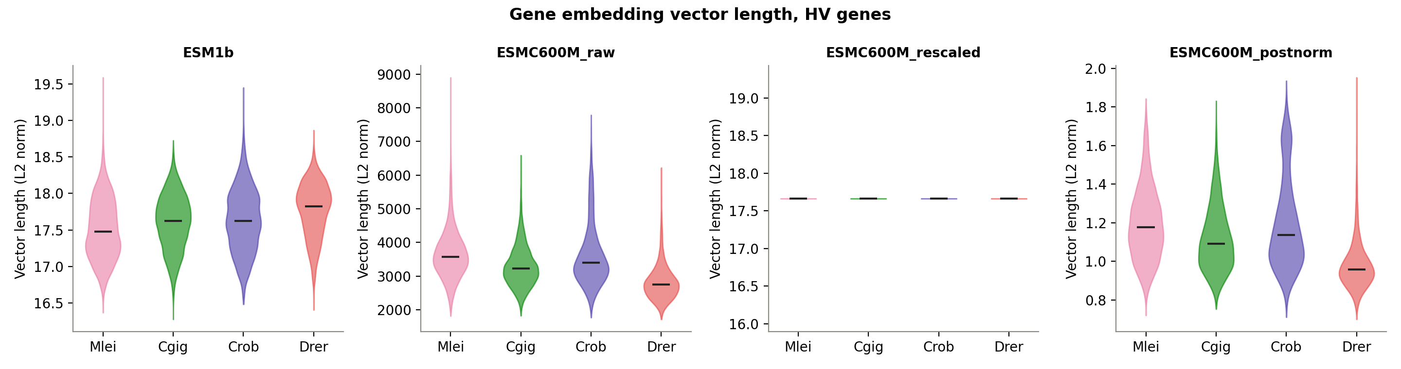
| Median length | Mnemiopsis | oyster | Ciona | zebrafish | spread (q95/q5) |
|---|---|---|---|---|---|
| ESM-1b | 17.5 | 17.6 | 17.6 | 17.8 | 1.07–1.08× |
| ESMC raw | 3,579 | 3,220 | 3,396 | 2,749 | 1.8–2.3× |
| ESMC rescaled | 17.7 | 17.7 | 17.7 | 17.7 | 1× |
| ESMC post-norm | 1.18 | 1.09 | 1.14 | 0.96 | 1.5–1.9× |
- Post-norm fixed the scale but not the variation. Lengths are now near 1, but still vary about 1.5–1.9-fold between genes, and zebrafish vectors are systematically shorter. That was also the pattern in raw.
- Length doesn’t follow protein length for ESMC (Spearman ρ 0.04–0.15 for raw and post-norm; −0.27 to −0.37 for ESM-1b). So the variation isn’t simply long proteins getting long vectors, which was one possible explanation for the shorter zebrafish vectors. A few dominant dimensions are the other candidate: the large gains from z-scoring (section 3.4) point that way.
3.2 Geometry
| ESM-1b | ESMC raw | ESMC rescaled | ESMC post-norm | |
|---|---|---|---|---|
| Effective dimensions (participation ratio) | 10.1 | 4.9 | 11.4 | 3.1 |
| Principal components for 90% of variance | 215 | 61 | 99 | 22 |
| Variance on the first component | 30% | 43% | 26% | 56% |
| First component vs vector length (abs r) | 0.50 | 0.96 | 0.02 | 0.91 |
| Species R² (Euclidean) | 0.075 | 0.131 | 0.117 | 0.146 |
| Mean similarity between all genes (cosine) | 0.96 | 0.85 | 0.85 | 0.76 |
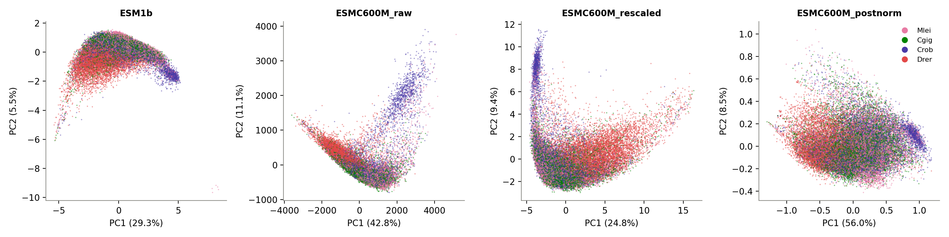
- Post-norm vectors are the most collapsed. More than half the variance sits on one direction, and about 3 directions do most of the work. That one direction still tracks vector length, as in raw.
- All three ESMC sets separate species more than ESM-1b does (species R² 0.12–0.15 vs 0.075). The ESMC authors expect some of this: the model encodes features correlated with the source organism, and in mean-pooled vectors this broad taxonomic signal can drown out local functional features (Candido et al. 2026, Appendix A.4.5.4, citing Ding & Steinhardt 2024). In the PCA, a block of Ciona genes forms a separate arm in raw and rescaled ESMC.
- Fewer cross-species neighbours, especially for zebrafish:
- Of each zebrafish gene’s 10 most similar genes, 35% come from other species with ESM-1b, vs 24–25% with any ESMC set (random expectation ≈ 75%).
- For the invertebrates the sets are closer: 39–49% for all.
3.3 Most-similar-gene ortholog test
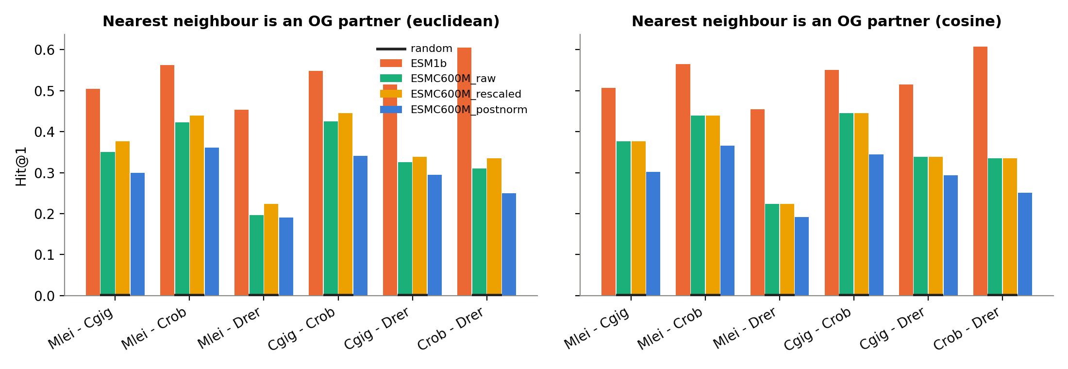
| Mean over 12 species pairs | hit@1 Euclidean | hit@1 cosine | hit@10 cosine |
|---|---|---|---|
| ESM-1b | 0.53 | 0.53 | 0.73 |
| ESMC raw | 0.34 | 0.36 | 0.51 |
| ESMC rescaled | 0.36 | 0.36 | 0.51 |
| ESMC post-norm | 0.29 | 0.29 | 0.43 |
| random | 0.00 | 0.00 |
| hit@1 (cosine) | ESM-1b | ESMC raw / rescaled | ESMC post-norm |
|---|---|---|---|
| Mnemiopsis → oyster | 0.48 | 0.34 | 0.28 |
| Mnemiopsis → Ciona | 0.53 | 0.40 | 0.34 |
| Mnemiopsis → zebrafish | 0.37 | 0.16 | 0.14 |
| oyster → Ciona | 0.55 | 0.45 | 0.35 |
| Ciona → zebrafish | 0.52 | 0.26 | 0.20 |
| zebrafish → Ciona | 0.69 | 0.41 | 0.30 |
- The order holds for every species pair: ESM-1b > ESMC raw/rescaled > ESMC post-norm.
- The gap is largest for zebrafish. Zebrafish → Ciona is 0.69 with ESM-1b vs 0.30 with post-norm.
- The OrthoFinder reference gives the same picture. ESM-1b 0.59 vs post-norm 0.29 (hit@1, Euclidean); Mnemiopsis pairs 0.55 vs 0.27.
3.4 Do standard fixes close the gap?
| hit@1, mean of 12 pairs | ESM-1b | ESMC raw (Oct 8) | ESMC post-norm |
|---|---|---|---|
| as delivered | 0.53 | 0.34 | 0.29 |
| unit length | 0.53 | 0.36 | 0.29 |
| z-score per dimension | 0.57 | 0.42 | 0.42 |
| top 2 directions removed | 0.61 | 0.47 | 0.43 |
| top 3 directions removed | 0.61 | 0.49 | 0.46 |
| best (top 3 removed, cosine) | 0.63 | 0.47 |
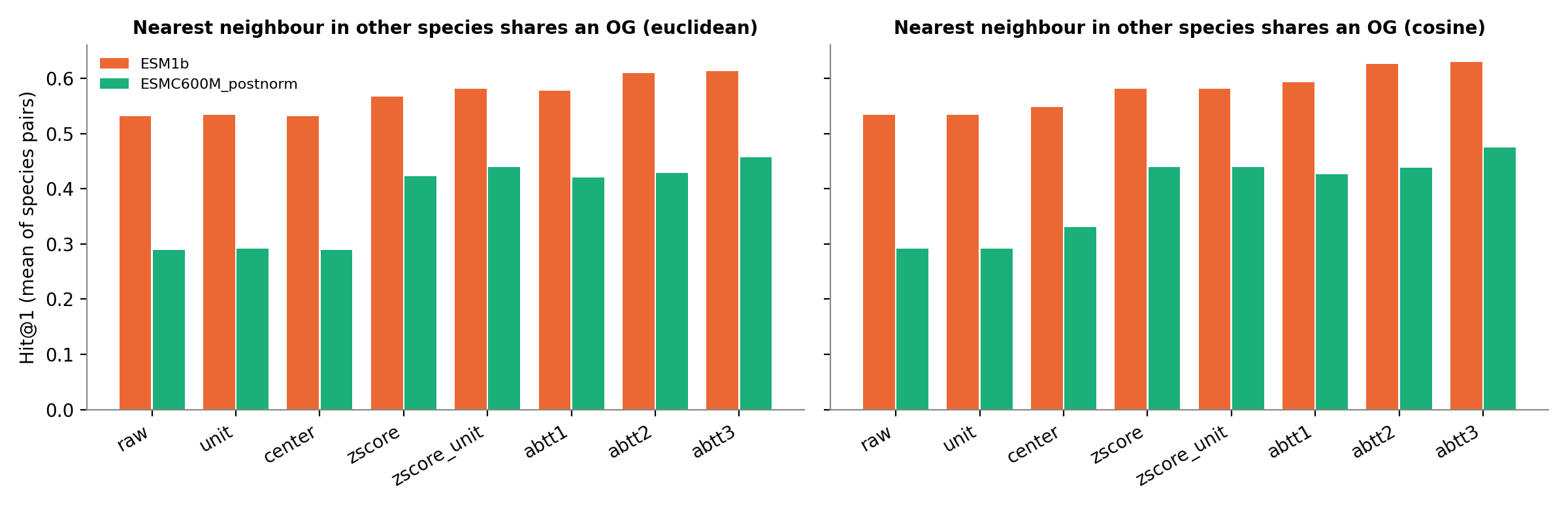
- Every fix helps ESMC more than ESM-1b, but none closes the gap. The best post-norm result (0.47) is below ESM-1b with no fix at all (0.53). Against OrthoFinder: 0.49 vs 0.59.
- The z-score fix brings both ESMC exports to the same 0.42. Z-scoring equalizes the spread of every dimension, and the two exports converge after it. So they differ mainly in how individual dimensions are scaled, which is what the final LayerNorm’s learned per-dimension weights do (section 1.1).
3.5 Macrogenes (from Oct 8)
| 4-species macrogene-only run | Recall | Precision | Recall, Mnemiopsis pairs |
|---|---|---|---|
| ESM-1b | 0.30 | 0.134 | 0.26 |
| ESMC raw | 0.15 | 0.054 | 0.13 |
| ESMC rescaled | 0.16 | 0.058 | 0.14 |
| ESMC post-norm | not run |
The embedding-level ranking (Table 7) matched the macrogene ranking for the three sets where both exist. So the most-similar-gene test predicts macrogene quality, and it is cheap enough to screen new embeddings before running SATURN. A post-norm SATURN run is in progress on the 6-species panel.
Interpretation
- ESM-1b stays ahead on every measure so far: embeddings alone, after any fix, and in SATURN’s macrogenes.
- The last layer of ESMC, read either way, is below ESM-1b.
- The extraction is now fully documented: final block, before (raw) or after (post-norm) the final LayerNorm, mean over residues, start/end tokens excluded, 2,000-residue limit.
- Reading after the LayerNorm, the convention that matches ESM-1b, made the results worse, not better.
- Still untested: intermediate layers, which for several protein language models carry more transferable information than the last layer. Those would settle whether the gap is about ESMC itself or about where it is read.
- The ESMC paper supports this directly:
- in ESMC 6B, functional organization (enzyme class by nearest neighbours) peaks at layers 50–60 of 80, while structure peaks in the final layers (Candido et al. 2026, Fig. 1D);
- for stability probes, the second-to-last layer beat the final layer, which “is projected to final sequence logits” (Appendix A.1.4).
- Those analyses are within one model and not cross-species, and the 600M layer profile isn’t shown, so they suggest where to look but don’t predict our result.
- One property is shared by every ESMC export: more species signal and fewer cross-species neighbours, especially for zebrafish. In SATURN this shows up as zebrafish genes set apart in their own macrogenes (Oct 8). This matches the taxonomic bias the ESMC authors describe for mean-pooled embeddings (Candido et al. 2026, Appendix A.4.5.4; Ding & Steinhardt 2024). Because ESMC’s training data are mostly metagenomic (largely microbial), animal lineages may be sampled unevenly, but we haven’t tested that.
Caveats
- Both references are sequence-based (eggNOG and OrthoFinder) and could favour a model whose similarity tracks sequence. A gap present before SATURN and surviving every fix is hard to explain this way.
- All ESMC sets keep residues 1–2,000; ESM-1b keeps residues 1–1,022. This affects 1–4% of proteins per species and can’t explain gaps of this size.
- Only the final layer has been extracted for ESMC. The FANTASIA files contain no other layers.
- All four sets use mean pooling. The ESMC paper shows that, with mean pooling, one broadly active feature can dominate cosine similarity between distant homologs (71% of it in their human vs Candida ATP8 example; max pooling reduced this). That example is in sparse-autoencoder feature space, not the dense vectors used here (Candido et al. 2026, Appendix A.4.5.1). Pooling choice is untested here.
- ESMC was trained in bf16 mixed precision (Candido et al. 2026, Table S3); both ESMC exports were run in fp32. This is a standard setup and isn’t expected to matter.
Next steps
Scripts
All in pipelines/scripts/saturn_embedding_comparison/.
| Script | What it does |
|---|---|
05q_convert_esmc_postnorm.py |
converts the post-norm export to SATURN gene embeddings (same gene bridges and isoform averaging as before) |
05r_esmc_postnorm_check_4sp.sh |
Pegasus job: 05q → 05f → 05i (eggNOG and OrthoFinder) |
05f_embedding_descriptives.py |
vector length, geometry, neighbour mixing, most-similar-gene test (--extra_model adds a set) |
05i_embedding_standardization_check.py |
the test after standard fixes (--esmc_dir, --reference) |
05e_rescale_esmc_embeddings.py |
makes the rescaled set |
05g_compare_runs_orthology.py |
macrogene ortholog benchmark (Oct 8) |
# Pegasus (job 603388, normal queue, 32 GB)
bsub -q normal -P dark_genes -R "rusage[mem=32000]" < scripts/05r_esmc_postnorm_check_4sp.sh
References
- Rives A. et al. (2021) Biological structure and function emerge from scaling unsupervised learning to 250 million protein sequences. PNAS 118:e2016239118.
- Candido S., Hayes T., Derry A., Rao R., Lin Z., Verkuil R., … Rives A. (2026) Language modeling materializes a world model of protein biology. bioRxiv, posted June 4, 2026. doi:10.64898/2026.06.03.729735. The primary ESMC paper: architecture (Appendix A.1.1, Table S1), training data and context (Tables S2–S3), layerwise analyses (Fig. 1D, Appendix A.1.4), pooling and taxonomic bias (Appendix A.4.5.1, A.4.5.4).
- EvolutionaryScale (2024) ESM Cambrian. https://evolutionaryscale.ai/blog/esm-cambrian
- Ding F., Steinhardt J. (2024) Protein language models are biased by unequal sequence sampling across the tree of life. bioRxiv.
- Miranda Perez I. (2026) Extraction details of the FANTASIA v4.1.1 and post-norm ESMC-600M exports (personal communication, Oct 2026).
- Rosen Y. et al. (2024) Toward universal cell embeddings: integrating single-cell RNA-seq datasets across species with SATURN. Nature Methods 21:1492–1500.
- Mu J., Viswanath P. (2018) All-but-the-top: simple and effective postprocessing for word representations. ICLR 2018. https://arxiv.org/abs/1702.01417
- Timkey W., van Schijndel M. (2021) All bark and no bite: rogue dimensions in transformer language models obscure representational quality. EMNLP 2021. https://aclanthology.org/2021.emnlp-main.372
- Emms D.M., Kelly S. (2019) OrthoFinder: phylogenetic orthology inference for comparative genomics. Genome Biology 20:238.
- Cantalapiedra C.P. et al. (2021) eggNOG-mapper v2. Molecular Biology and Evolution 38:5825–5829.